Bayesian Conjugate Updating and Hierarchical Partial Pooling

An Undergraduate Guide to Normal-Normal & Beta-Binomial Shrinkage, Empirical Bayes Credibility, and Fair Benchmarking

1 The Small-Sample League Table Paradox

Suppose you are comparing outcome rates across hundreds of schools, hospitals, or regional clinics. Which institutions appear at the very top (best) and very bottom (worst) of an unadjusted ranking table? Almost invariably, the smallest institutions with the fewest observations (\(n_j = 1\) or small denominator \(m_j\))!

Because sampling variance scales inversely with sample size (\(\mathrm{Var}(\bar{y}_j) \propto 1/n_j\)), small cohorts experience large random swings from transient shocks. Hierarchical Bayesian Modeling and Conjugate Partial Pooling provide a mathematically exact solution that every undergraduate statistics student can master from first principles.

2 Step 1: Normal-Normal Conjugacy and the Empirical Bayes Credibility Weight \(w_j\)

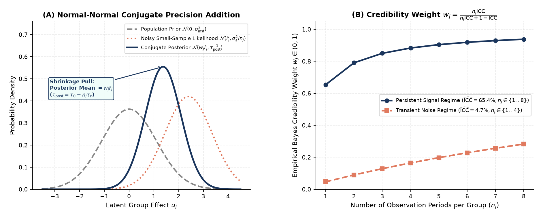
For continuous outcomes where group \(j \in \{1, \dots, J\}\) has a persistent latent effect \(u_j \sim \mathcal{N}(0, \sigma_{\mathrm{inst}}^2)\) and \(n_j\) noisy observations with residual variance \(\sigma_\varepsilon^2\), Normal-Normal conjugacy tells us that prior precision \(\tau_0 = \sigma_{\mathrm{inst}}^{-2}\) and data precision \(\tau_{\mathrm{data}} = n_j \sigma_\varepsilon^{-2}\) add linearly:

\[u_j \mid \bar{r}_j, \sigma_{\mathrm{inst}}^2, \sigma_\varepsilon^2 \sim \mathcal{N}\!\left(w_j \bar{r}_j, \;\; \frac{1}{\sigma_{\mathrm{inst}}^{-2} + n_j \sigma_\varepsilon^{-2}}\right), \qquad w_j = \frac{n_j \, \mathrm{ICC}}{n_j \, \mathrm{ICC} + (1 - \mathrm{ICC})},\]

where \(\mathrm{ICC} = \sigma_{\mathrm{inst}}^2 / (\sigma_{\mathrm{inst}}^2 + \sigma_\varepsilon^2)\) is the Intraclass Correlation Coefficient (estimated from the marginal likelihood via Restricted Maximum Likelihood, REML, in an Empirical Bayes plug-in approach):

• When Transient Noise Dominates (\(\widehat{\mathrm{ICC}} = 4.7\%\) across \(n_j \in \{1, \dots, 4\}\) quarterly waves): A single-wave spike (\(n_j = 1\)) receives reliability weight \(w_1 = 0.047\), shrinking \(95.3\%\) of its extreme deviation back toward the covariate-adjusted population expectation!
• When Persistent Signal Dominates (\(\widehat{\mathrm{ICC}} = 65.4\%\) across \(n_j \in \{1, \dots, 8\}\) annual cycles): An institution observed over \(8\) years receives \(w_8 = 0.938\), allowing its consistent multi-year record to speak for itself.

3 Step 2: Beta-Binomial Conjugacy on \((0, 1)\) and Complexity-Adjusted Benchmarking (aPTA)

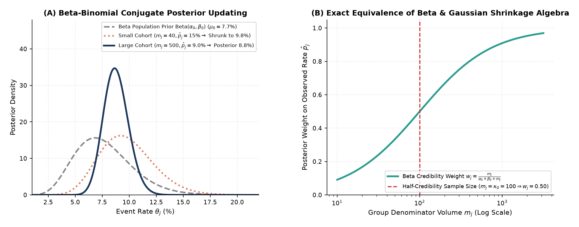
What if the outcome is a bounded proportion \(p_j \in (0, 1)\), such as a 30-day complication or readmission rate (\(y_j\) events out of \(m_j\) cases)? Placing a conjugate \(\mathrm{Beta}(\alpha_0, \beta_0)\) prior (with prior mean \(\mu_0 = \alpha_0 / \kappa_0\) and concentration \(\kappa_0 = \alpha_0 + \beta_0\)) on \(\theta_j\) under a \(\mathrm{Binomial}(m_j, \theta_j)\) likelihood yields an exact Beta posterior:

\[\theta_j \mid y_j \sim \mathrm{Beta}(\alpha_0 + y_j, \;\; \beta_0 + m_j - y_j), \qquad \mathbb{E}[\theta_j \mid y_j] = \underbrace{\left(\frac{m_j}{\kappa_0 + m_j}\right)}_{w_j} \hat{p}_j + \underbrace{\left(\frac{\kappa_0}{\kappa_0 + m_j}\right)}_{1 - w_j} \mu_0.\]

Notice the exact algebraic symmetry between the Gaussian and Beta shrinkage formulas: when a group’s sample volume \(m_j\) equals the prior concentration \(\kappa_0\), the credibility weight is exactly \(w_j = 0.50\). For continuous covariate regression on \((0, 1)\), Beta regression models the conditional mean directly on the rate scale (using the Smithson-Verkuilen boundary compression \(y' = [y(N-1)+0.5]/N\), which acts like a \(0.5\) boundary pseudo-count).

3.1 Fair Decision Theory: Static Cutoff \(T\) vs. Complexity-Adjusted Curve \(T(s_j)\)

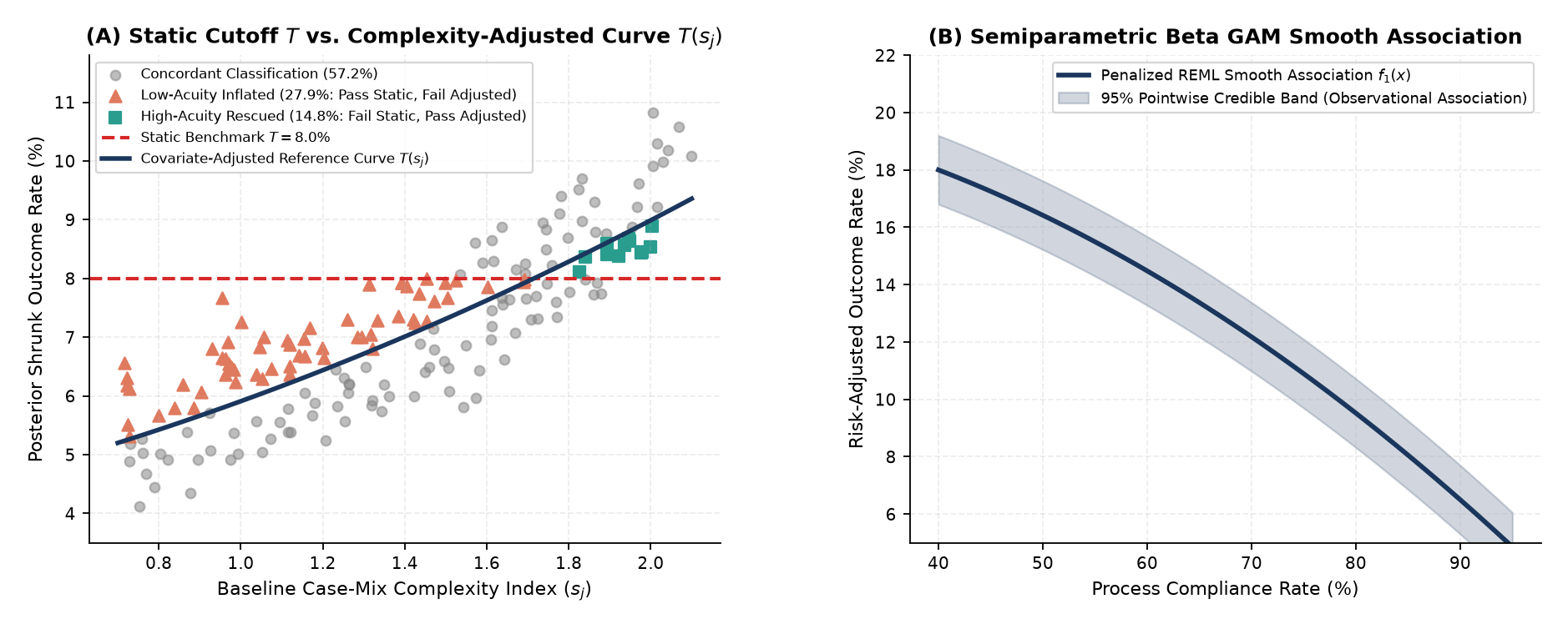
Evaluating each group’s posterior Probability of Target Attainment (\(\mathrm{PTA}_j = P(\theta_j < T \mid \mathrm{Data})\)) against a single flat cutoff \(T = 8.0\%\) is unfair when baseline case-mix complexity \(s_j\) varies strongly across groups (\(r = 0.76\)). Benchmarking each group against the conditional expectation curve \(T(s_j)\) at its own complexity index (Adjusted \(\mathrm{aPTA}_j\)) reclassifies \(42.8\%\) of institutions (\(27.9\%\) low-complexity inflated and \(14.8\%\) high-complexity rescued), while reminding analysts to audit whether complexity codes themselves are inflated by reporting intensity.

Conjugate / Regression Family	Posterior Distribution	Credibility Weight \(w_j\)	Key Pedagogical Lesson
Normal-Normal Hierarchy (Unbounded Outcomes)	\(\mathcal{N}\!\left(w_j \bar{r}_j, \, (\tau_0 + n_j \tau_\varepsilon)^{-1}\right)\)	\(w_j = \frac{n_j \, \mathrm{ICC}}{n_j \, \mathrm{ICC} + 1 - \mathrm{ICC}}\)	Precision adds linearly; small \(n_j\) and low \(\mathrm{ICC}\) trigger strong shrinkage
Beta-Binomial Hierarchy (Bounded Counts \(y_j / m_j\))	\(\mathrm{Beta}(\alpha_0 + y_j, \, \beta_0 + m_j - y_j)\)	\(w_j = \frac{m_j}{\alpha_0 + \beta_0 + m_j}\)	Prior pseudo-counts \(\kappa_0 = \alpha_0 + \beta_0\) stabilize small denominators \(m_j\)
Complexity-Adjusted Decision Rule (\(\mathrm{aPTA}\))	\(P(\theta_j < T(s_j) \mid \mathrm{Data})\) vs. Static \(P(\theta_j < T)\)	Reclassifies \(42.8\%\) of groups across complexity \(s_j\)	Separates group performance from baseline cohort severity (subject to coding audits)

4 Exploring Further: Research Directions

Research Track	Core Question to Investigate	Tools & Methods
1. Empirical Bayes vs. Full MCMC Hierarchy	When does plugging in REML point estimates \((\hat{\sigma}_{\mathrm{inst}}^2, \hat{\sigma}_\varepsilon^2)\) underestimate posterior rank uncertainty compared to full Hamiltonian Monte Carlo (Stan)?	Empirical Bayes vs. Full Bayes, CmdStanPy / PyMC
2. Auditing Measurement Error in Complexity \(s_j\)	How does random or systematic upcoding in the complexity index \(s_j\) bias complexity-adjusted rankings, and how can instrumental variables correct it?	Measurement-Error Models, Sensitivity Analysis
3. Semiparametric Beta Generalized Additive Models	How do penalized thin-plate splines and tensor-product smooths \(\mathrm{ti}(x_1, x_2)\) capture nonlinear interaction surfaces on \((0, 1)\)?	Penalized Likelihood Splines, Beta Regression